
Tapping Mode Atomic Force Microscopy
Roger Robbins
January 30, 2010
Table of Contents
- Tapping Mode Atomic Force Microscopy
- Operation Manual
- Purpose
- Operational Capabilities
- Tapping Mode Concept and Hardware
- Tapping Mode Step-by-step Detailed Instructions
- Mounting AFM Tip Chip on Holder
- Aligning Laser to Cantilever and Detector
- Step 1. Start the AFM Software to Power up and Initialize the AFM System
- Step 2. Set the system to tapping Mode
- Step 3. Move the Stage back so the area under the AFM head is clear of the sample stage
- Step 4. Align the Laser Beam to the Cantilever
- Step 5. Align the Reflected Laser Beam to the Detector
- Vacuum Clamp your Sample to the Sample Stage
- Focus on cantilever and Sample
- Set up the Driving Frequency for the Cantilever
- Set up File Save Path and Thumbnail directory
- Find the Region of Interest on the Sample
- Set up Initial Operating Parameters
- Engage Probe
- Adjust Parameters to Optimize Image
- Capture Image
- Save Image
- Shutdown Procedure
- Log Out of Logbook
Purpose
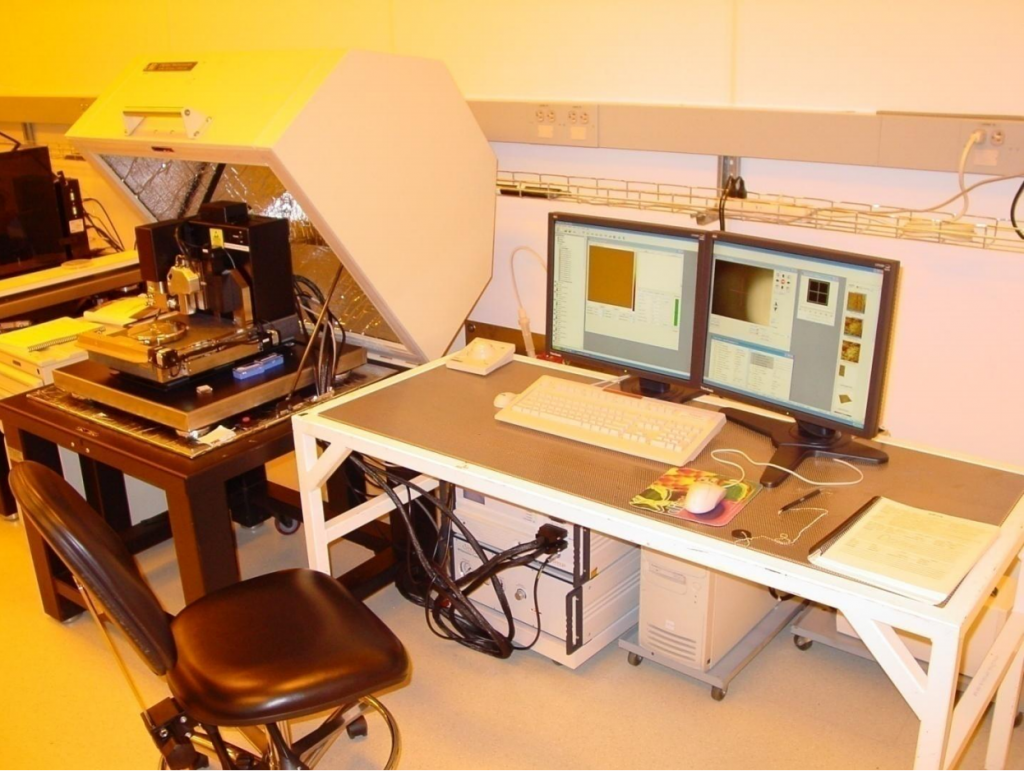
The intent of this document is to present the basic operation instructions for using the UTD Cleanroom Atomic Force Microscope (AFM) in the tapping mode. The Cleanroom AFM is a Veeco, Model 3100 Dimension V Atomic Probe Microscope, fondly called our AFM for short. The principal upon which this tool images a surface is that it scans a very sharp probe point across a sample surface and monitors the vertical movement of the probe. Multiple scans are collected into a graph until a topographical image emerges. Because of the sharp point and precision tooling, this system can image and measure features as small as single atomic plane steps in a crystal surface. It is heavily used to measure feature depths, lengths, widths, surface roughness, and image highly magnified surface features. In particular, the tapping mode of operation follows the surface with the probe tip oscillating up and down, just tapping the surface, which lessens the likelihood of scratching a trench in the surface, so it is ideal for soft surfaces like polymer materials and delicate nano structures – by the way, it also works on hard surfaces.
Operational Capabilities
This document is focused on Tapping mode imaging, but just so you will know in case you might need other capabilities, I will list a few of them, but with small changes or additions of adapters, etc, the tool can do even more than the following listing.
- Contact Mode Surface Imaging: Normal method of obtaining surface morphology by dragging the tip over the surface with the tip in contact with the surface. This is a common mode of operation and the AFM tips for this mode are cheap. The surface needs to be “hard” so the dip will not scratch the surface.
- Tapping Mode Imaging: Most popular mode of obtaining surface morphology by scanning the surface with the tip oscillating up and down and just tapping the surface (at ~300KHz) lightly. This is a common method for use in observing a surface that is “soft” and easily scratched by dragging the AFM tip while it is in contact with the surface.
- Scanning Tunneling Microscopy: Method of obtaining very high magnifications by scanning the tip over the (electrically conducting) surface and maintaining the height of the tip above the surface constant by monitoring the amplitude of the quantum tunneling current between the tip and the conducting surface of the sample. The tip is moved up and down over the topography of the surface by piezo actuators using feedback signal from the tunneling current to maintain the tunneling current constant.
- Interleaved Lift Mode: General Method of measuring electrical or magnetic field strength just above the surface by tapping mode measurement of surface topography, saving the height data for the scan and then lifting the tip slightly above the surface and re-scanning the same trace. While in the elevated scan the tip can observe electrical or magnetic fields by monitoring the tapping amplitude, phase, or frequency modulation of the resonance frequency due to the fields. For magnetic sensing, the tip has to be magnetized prior to the imaging. Electrical fields require a bias of the tip or the sample.
- Lateral force microscopy: In this measuring scheme, the tip is dragged across the surface in a direction perpendicular to the tip cantilever so the tip moves sideways. The surface drag on the tip causes the cantilever to twist on its axis, so the detector uses the 4- quadrant detector signals from the left pair and right pair as the tip’s twisting motion detectors. This yields a map of friction between the moving dragging tip and the surface.
- Magnetic Force Microscopy: This technique maps the magnetic force on the tapping mode tip and produces an image consisting of the relative changes in magnetic force on the tip. The mechanical methodology in producing this image consists of scanning the tip across the surface in normal tapping mode to record the surface topography over one scan and then rescans that line with the tip lifted by some distance and detecting the shift in tapping phase compared to the tapping driving signal. The phase is shifted as the magnetic tug on the magnetized tip causes the tapping timing to change slightly due to the changes in magnetic force. It does not measure absolute magnetic field strength – only the relative changes.
- Electric Force Microscopy: This measurement follows the format of the above MFM technique, however it requires that there be an electric bias on the tapping mode AFM tip and that the sample have regions of electric fields above the surface to create an image. This also uses the Lift mode to retrace each scan at an elevated distance so that the electric field force can cause a similar phase shift in the tapping motion.
- Other Modes: There is a poster on the wall behind the SEM that outlines a multitude of measurement methods.
Tapping Mode Concept and Hardware
In order to help the reader understand the physical layout of the AFM head, a short description will be given in the following sections.
The internal layout of the AFM head is shown in Figure 1. In this clever design, almost the entire working part of the AFM is contained in this enclosure. The head includes the piezo system to follow the terrain in the Z-axis as well as generating the x-y scans by bending the z-piezo element with pairs of side mounted piezo elements which expand and contract in such a way as to bend the z-piezo in arcs in both x and y directions. In the figure, the optical configuration is depicted to show the cantilever laser aiming mechanism as well as the steering mirror adjustment to direct the reflected laser beam from the cantilever to the quad detector which detects cantilever deflection.
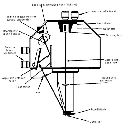
Figure 1. Illumination of the interior of the Veeco Dimension SPM Head showing the laser path including the alignment knob functions.
Tapping Mode Step-by-step Detailed Instructions
The following paragraphs describe the AFM Tapping Mode operation in detail with explanations for each step. The material is arranged in the order required to operate the system and capture an image in the Tapping Mode. Appendix A gives a step-by-step summary listing of operational steps with a very short description in the order of procedural flow to produce an image.
1. Mounting AFM Tip Chip on Holder
There are two operations that seem to create difficulties for new AFM users: One is loading the probe tip into the tip holder and the other is aligning the signal laser to the tip cantilever once it is mounted onto the AFM head. Both of these operations need a bit of practice before they can be done smoothly. The following description outlines the detailed steps required in mounting the probe in its holder, affixing it to the AFM head and then aligning the probe laser to the probe tip and detector.
Step 1. Gather Probe Tip and Tools
The AFM probe tip mounts in a small tray on a small printed circuit card which connects the probe to various voltages used to create multiple modes of operation, (Figure 2). This fixture clamps the probe firmly under a spring clip and cants the probe at the proper angle for imaging. The fixture also contains a piezo stack which can vibrate the tray and stimulate the probe to oscillate for the Tapping Mode
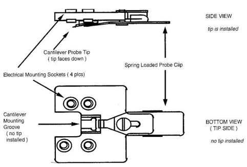
Figure 2. Cantilever holder showing mounting pins, tray (Groove) for the probe tip and spring clip for clamping the tip in the tray.
Figure 3 shows the tip holder fixture, the gel-pak box of probe tips, and a pair of very sharp tweezers for handling the probe. The tip holder fixture is a highly useful aid in holding the tip holder to aid in the probe mounting process. The probes usually come in a gel-pak box which securely holds the probe tips on top of a slightly sticky gel that allows one to pick up the probes with a sharp tweezers.
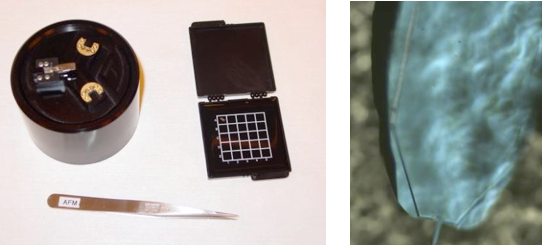
Figure 3. Assemblage of components in preparation for mounting a probe tip in the probe holder and an angle shot of the cantilever chip to show the beveling of the end and edges.
Step 2. Mounting the Probe Tip in the Probe Holder
The process of picking up the probe and setting it into its tray on the probe holder is a bit tricky and requires a rather steady hand. The process details are listed below:
A. Set the probe holder onto the pins of the holder fixture on the mount with the plastic post filling the cutout in the probe holder (Figure 4). Insure that the holder is seated on the pins. Then, while holding the probe holder seated with two fingers, grasp the spring clip with two other fingers and pull it gently back onto the rear ledge of the probe tray.
B. Pluck the probe chip out of the gel-pak box with a pair of very sharp tweezers by grasping the chip body and tilting it away from the gel. It will easily come off. The cantilever is located at the end of the probe chip that has beveled corners.
C. Place the probe in the tray with the cantilever facing outwards.
D. With two fingers holding the probe holder in place, grasp the spring clip with two other fingers, press slightly downwards to lift the front of the clip above the probe, and slide the spring clip forward to its limit and then allow it to come to rest on the probe chip and clamp it to the tray. See the video clip in Figure 4 for example.
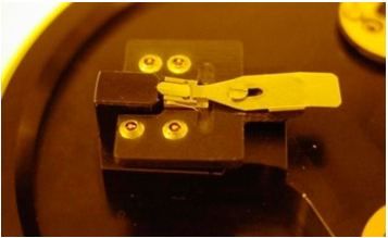
Figure 4. Loading AFM tip into holder Note that the standard probe holder is mounted on the pin block with the raised post. This helps keep the probe from falling on its cantilever and breaking if it accidently falls off the front of the tray.
Step 3. Alignment of the Probe Chip in the Holder Tray
Now that the probe chip is clamped in the holder tray, the next operation is to align the chip parallel to the edges of the tray. This is done by setting the fixture with the probe mounted in the tray under the handy illuminated-field low power microscope sitting on the SEM/AFM sample prep table. Once the probe is visible under the microscope, scoot the probe chip parallel to the edges of the tray with the point of your very sharp tweezers. The little video clip in Figure 5 shows this operation. The scooting operation requires very steady hands and a very controlled scoot of only a few microns. The goal is to have the probe chip sitting in the center of the tray with its sides parallel to the tray edge and its rear end up against the back edge of the tray. Figure 5 shows the probe chip aligned in the center of the tray and the spring clip clamping it firmly to the tray. If your fingers turn out to be a little jittery, just place a finger of the other hand on the tweezers to steady it. Also contacting the edge of the holder fixture with your tweezers-wielding hand will steady it for the delicate motion required.
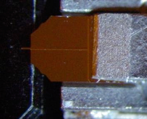
Figure 5. The image shows the probe chip centered and its edges parallel with the walls of the tray.
Step 4. Probe Holder Attachment to Head
In order to mount the probe onto the AFM driver head, the head must be removed from the z- stage, tilted up to reveal the probe pins, the holder plugged onto the pins and the head replaced on the z-stage. This is simple enough, but there are a couple of practical guidelines to follow to avoid dropping or damaging things. First, make sure that you are wearing gloves that fit the ends of your fingers very snugly. This avoids the trap of having the gloves interfere with holding the probe holder and placing the probe holder on the head pins. The other thing to be careful with is bending the head cables very sharply while plugging the probe holder onto the head. The wires are very delicate and if they break because of fatigue of bending, then the repair is costly and requires a long down time. Figure 6 shows a video of proper handling of the probe head. Please be very gentle and careful in plugging the tip holder into the head pin base – excessive sidewise force could break the z-piezo element. Repair is slow and very costly.
Figure 6. Disconnecting AFM head, placing the tip holder on pins, and remounting the AFM head Note the asymmetric pin locations designed to allow the probe holder to fit only in the proper orientation. Make sure that the probe holder is seated flush against the head pin base, but be very gentle and do not push the pin base sideways – the z-piezo could break with excessive force. The video clip shows the mounting sequences. Note that the clamping screw for the AFM head has reverse threads – turn CCW to clamp the head and CW to release it.
2. Aligning Laser to Cantilever and Detector
This is the step where the operator aligns the laser beam to the cantilever so that the AFM can measure the cantilever deflection as it encounters surface topography during its scan along the sample surface. The object of alignment is to position the laser beam on the tip of the cantilever and then adjust the reflected laser beam onto a split diode photo detector, which produces a voltage proportional to the deflection of the cantilever. A rough sketch of this alignment geometry is shown in Figure 7.
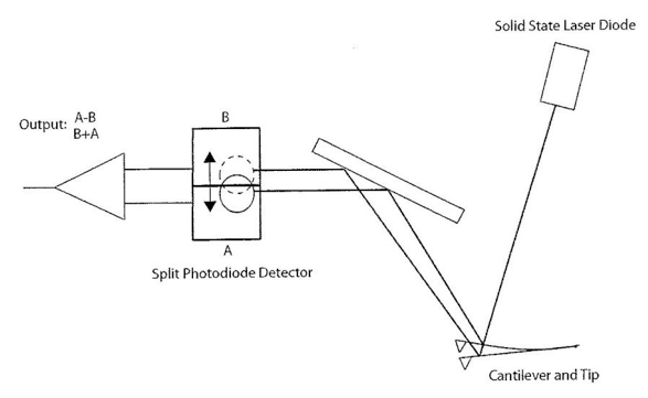
Figure 7. Sketch of laser alignment to probe cantilever and then to the split photodiode detector. This laser and detector are located inside the AFM head and the alignment is controlled by knobs on the head.
Step 1. Start the AFM Software to Power up and Initialize the AFM System
- Click on the microscope icon to start the AFM software
- When the Dimension V software starts up, there will be an icon in the upper left tool tray that also looks like a microscope. Click on that to power up and initialize the software and the hardware.
- Click on “File” in the upper left task bar and then click on “Open Workspace”. Find your workspace and open it.
- When the workspace opens, it will have many of your preferences open automatically; however they may be placed in strange places on the screen because Windows remembers how the previous user arranged the windows. So you might have to rearrange them to your liking. (Figure 8 shows a convenient and useful arrangement).
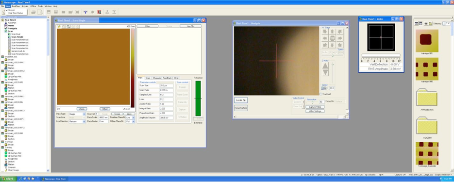
Figure 8. Useful arrangement of control windows to run the AFM
- Click on Acquire and open the scan-single window if it does not open automatically.
- Click on Acquire and open the Navigate window if it does not open automatically.
- Click on Acquire and open the Meter window if it does not open automatically.
- Click on “View” in the upper left task bar and select “Browse” to open the thumbnail index at the far right side of the right monitor screen.
Step 2. Set the system to tapping Mode
- Since we are planning to use the Tapping mode of operation, we should set the mode up now.
- If you don’t yet have the scan-single window open, click on the Real Time menu at the upper left menu line and then click on Scan-Single to bring up the Real Time 1 Scan-Single window as shown in Figure 9 below.
- Note that sometimes at this point, the software will ask permission to initialize the “Stage” – (in this case the vertical stage that moves the AFM head up and down).
- Click “OK” and “Yes” and then answer OK to all the other little boxes that pop up along the way.
- Click on the “Other” tab in the lower right menu listing
- On the Microscope Mode line, click on whatever name is in the box to call down a menu listing of modes and click on “Tapping”. This will set up the system to implement the tapping functions.
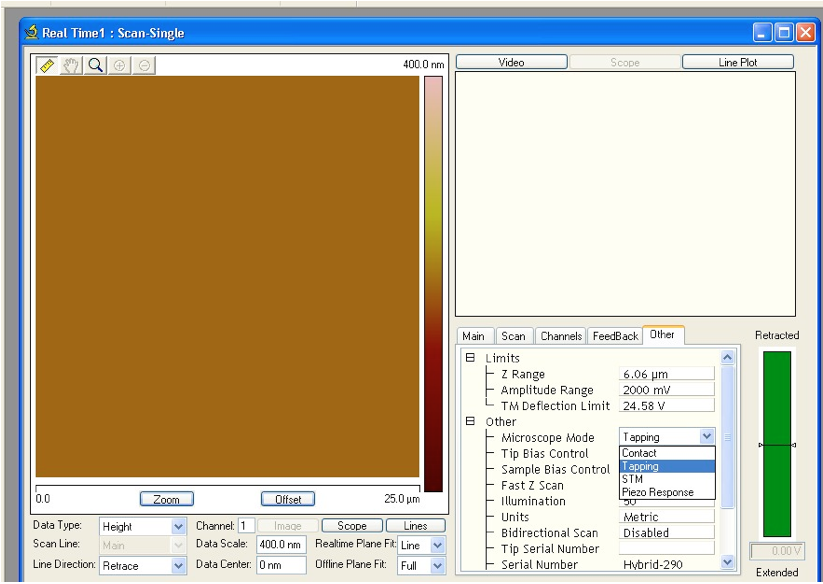
Figure 9. Scan-single window with menus to define the mode of operation from the “Other” tab – note the Microscope Mode: “Tapping”.
Step 3. Move the Stage back so the area under the AFM head is clear of the sample stage.
- The stage can be controlled from the software by opening the navigate window (Figure 10). Note that the AFM tip has to be plugged into the AFM head before the stage can be moved from the software.
- Click on the Down arrow under the XY Stage box to move the stage out from under the AFM head if necessary. This will reveal a circle of light on the granite table from the optical microscope and also a red spot from the laser beam. (See Figure 11 below.) You can place a white paper under the AFM head to help see the laser spot inside the circle of white light from the microscope.
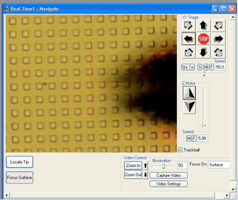
Figure 10. Navigate window in the AFM software. Note the XY Stage box with the motion arrows. Clicking and holding the left mouse button down will continuously drive the stage. The number under the “Speed” box sets the stage speed (0 – 100).
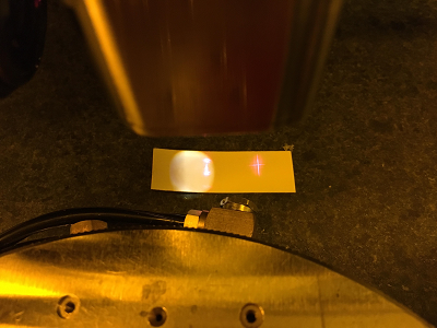
Figure 11. The stage position allowing the white light from the microscope to shine on the granite table to allow better alignment of the cantilever laser to the cantilever via shadow profile on the table. Note the white paper under the AFM head to improve visibility of the laser spot and cantilever shadow.
Step 4. Align the Laser Beam to the Cantilever
Step 1. Place a white paper under the laser head on the granite table to more clearly reveal the circle of white light from the microscope. Inside the circle of light should be a red dot from the laser. If it is not there you will have to turn the laser positioning knobs on the top of the AFM head to move it back into the light circle.
Step 2. Adjust the Right Rear knob on the top pair of knobs to bring the laser spot to the right edge of the light circle until it just disappears. Then bring it back so that it is only partially obscured.
Step 3. Adjust the Front Left knob to sweep the laser spot forward and backwards until the laser spot again disappears and then reappears from under the cantilever shadow. Center the cantilever shadow in the laser spot.
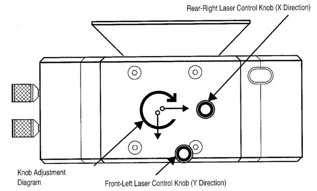
Figure 12. Layout of AFM Head from top. Top adjustment knobs adjust the laser alignment to the probe cantilever. Knobs on the left side align the reflected laser beam to the detector. If you turn the top knobs in the direction of the circular arrow, the laser spot will move in the direction of the corresponding linear arrow.
Step 4. When the cantilever shadow is centered in the laser spot, again adjust the top right rear knob to run the cantilever shadow almost out of the laser spot. The resulting laser spot shadow should have a bright red dot in its center and a fringe of red light on either side, (Figure 13). This is the proper centering of the laser over the cantilever. Remove the paper from the granite table.
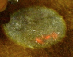
Figure 13. Circle of light with laser spot and cantilever shadow at right side. Note the diffraction maximum in the center of the shadow and the fractional laser spot on either side of the cantilever shadow.
Step 5. Note the green bar graph under the 4 square split photo diode detector schematic on the right AFM screen, Figure 14. At proper alignment of the normal OTESP cantilever probe, the voltage should read between 4 and 6 volts. This voltage level depends on the type of cantilever and whether it is coated with an optically reflective material.
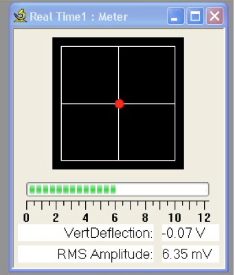
Figure 14. Meter indicator showing green bar graph depicting the proper amount of signal from the laser beam reflecting from the AFM cantilever (Tip type = OTESPa). Tapping mode should have the laser spot set at the center of the cross. Contact mode requires the red dot to be set on the vertical line at -2 volts Vertical Deflection.
Step 5. Align the Reflected Laser Beam to the Detector
The objective of this step is to center the reflected laser beam over the gap between the split photo diode detectors. When the laser spot is over the gap between the upper and lower split diode detectors, the voltage detector logic can very accurately determine vertical movement of the spot by finding the difference in voltage between the voltage sum of the upper pair and lower pair of detectors. The same advantage is had in the horizontal axis by taking the difference between the left and right pair of detectors.
For the Tapping Mode, adjust the red spot location on the photodiode detector depiction window to the horizontal gap line and vertical gap line intersection at 0 V using the two knobs on the lower left side of the AFM head as shown in Figure 15.
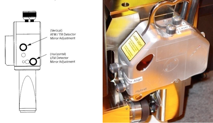
Figure 15. Side view from the Left of the AFM head showing the two knobs used to move the side mirror. Adjust them until the red dot on the screen lines up with the vertical gaps between the four sensors. A photograph of the AFM head is shown at the right.
3. Vacuum Clamp your Sample to the Sample Stage
Lay your sample over the vacuum port close to the edge of the round sample stage and flip up the Vacuum Switch on the upper console (Figure 16). For small samples the tiny beveled and threaded hole next to the upper edge of the round stage is the vacuum port that will clamp your sample to the stage sufficiently to make good AFM images.
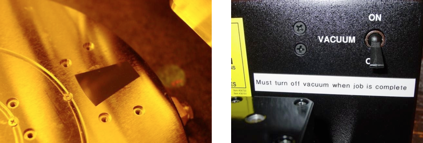
Figure 16. Location of sample vacuum port on round stage (under wedge shaped sample at Left). Vacuum switch is on the upper right of the console above the stage (Right).
4. Focus on cantilever and Sample
Step 1. Ensure that the probe tip is high enough to move the XY Stage under it and then move the stage so that the AFM tip is over the sample by clicking and holding on the appropriate arrows in the Navigate window under “XY Stage.”
Step 2. Lower the AFM head until the AFM tip is about 1 mm above the surface of your sample using the down arrow under the Z-Motor window inside the Navigate window (Figure n). Note: You can use the high speed setting (90) as you approach the surface, but when you get close, stop and slow the decent by setting the speed to Medium or Slow. DANGER: You can crash the piezo actuator into your sample if you hit it at high speed – this will cost a lot in repairs.
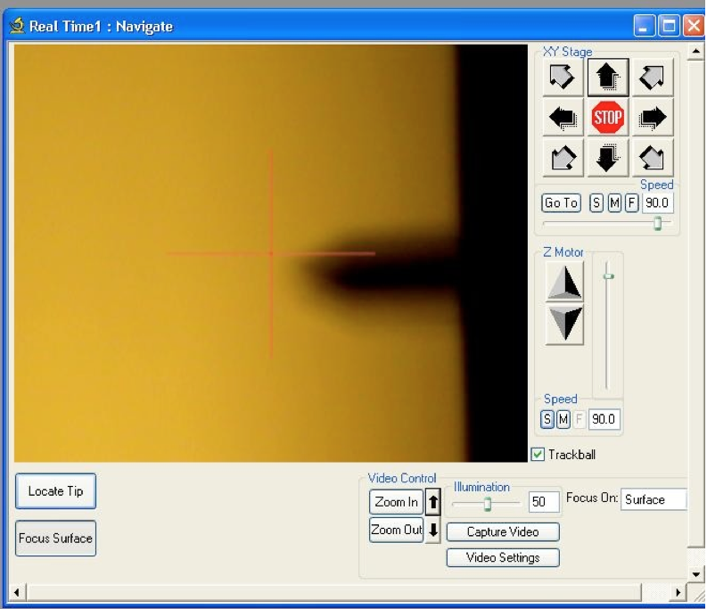
Figure 17. Navigate window showing XY Stage and Z Motor sub-windows for controlling the stage location and the height of the AFM head. Also shown in this image are the microscope Zoom controls: Arrows allow fractional up/down zooming; clicking on the Zoom boxes moves the zoom all the way up or down.
Step 3. When the AFM head is lowered and the cantilever is about 1 mm over the sample, the video screen in Figure 17 will be illuminated by the optical microscope’s lamp and you should see the silhouette of the cantilever in the screen. If the image is not there, click the “Zoom Out” button and you should for sure see the cantilever. ACTION: Click on the Locate Tip button under the video screen. Your job is to click on either the up or down arrow to move the Focus so that the tip comes into focus. Take care here to not crash the tip into the sample – go slow. Note that you will need to find an accurate focus at the point of the tip – zoom to high magnification for final focus adjustment (Figure 18).
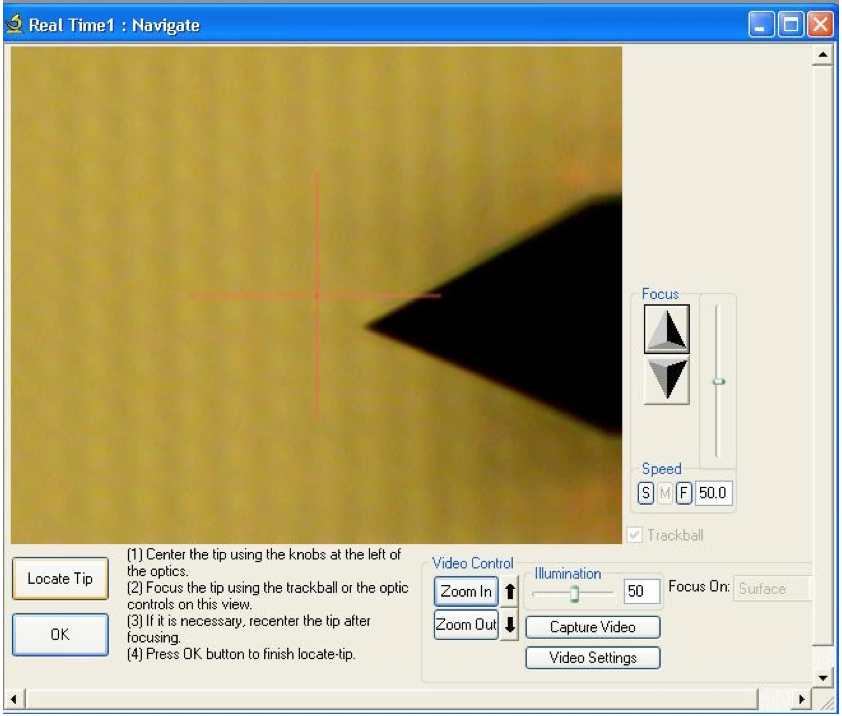
Figure 18. Focus on tip and position tip just off of the center of the red alignment cross.
Step 4. Center the point of the tip near but not on the center of the cross in the video screen using the two knobs on the video camera housing to the far left of the AFM head (see Figure 19 above).
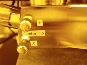
Figure 19. Alignment knobs on optics housing to center the tip image in the video camera’s screen
Step 5. Click on the OK button to complete the tip focus and set the microscope to a new focus 1 mm below the tip. This is a set-up reference configuration for automatic landing of the tip later.
Step 6. Click on the Focus Surface button and then click on the down arrow under the Z-Motor sub-window (formerly Focus sub-window) until the surface of your sample comes into focus. Also be accurate in your focus at this step.
Step 6a. If your sample surface is polished to a specular finish, you will not be able to see the surface. In this case you must select the “Focus on Tip Reflection” option from the Focus option menu in the lower right region of the Navigate window and then drive the optics further towards the sample and find the reflected image of the tip. Focus accurately here as well. (See Figure 17 above to locate the various buttons and menus).
5. Set up the Driving Frequency for the Cantilever
This step activates the piezo element under the probe and causes the cantilever to begin oscillating. The calibration operation sweeps the frequency from min to max to find the resonance frequency of the cantilever by finding the frequency at the maximum amplitude of cantilever oscillation from the Split Diode Photo Detector.
Step 1. Click on the blue tuning fork icon at the top of the left screen. This brings up a new overlay window (Figure 20) that contains myriads of parameters and two graphs.

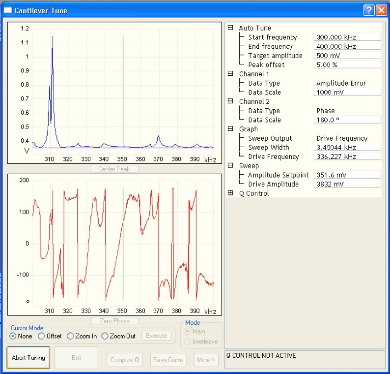
Figure 20. Cantilever Tuning window showing start and end frequency setup parameters and frequency spectrum with cantilever resonance peak. Click on Auto Tune to execute the tuning function and click Exit when it completes.
Step 2. Input the Start and End frequencies to span the resonant frequency listed on the probe gel-pak box label. Set the cantilever oscillation amplitude to 500 mV.
Step 3. Click on the Execute button at the lower left of the window and allow the software to find the resonance frequency and set the driving frequency to 5% below the resonance peak. (Figure 21)
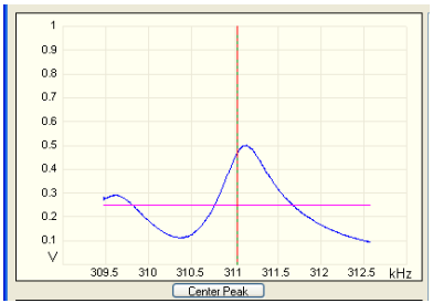
Figure 21. Calibration of resonance curve to set amplitude set 500 mV and offset driving frequency (at vertical line) by -5% of peak height to stabilize resonance and optimize performance.
Step 4. When the tuning process is complete, click on EXIT to quit.
At the conclusion of this step, you are ready to set up the scan parameters and begin scanning an image.
6. Set up File Save Path and Thumbnail directory
Before proceeding further, this is a good time to set up the file path to save your AFM images. The software remembers where to save images from the last user and if you forget to set up the path for your images, they will “disappear” into someone else’s directory.
- To set the path, pull down the “Real Time” menu on the top task bar and click on the
- “Save to…” choice.
- In the “Save to…” menu box, set the file path to your directory on the D:imagesyourname directory, or on your memory stick.
- You can also set a file name to which the software will attach sequence numbers to create a series of files with sequentially numbered file names with the same name (you could put the date as the reference name for example).
- To set up the thumbnail directory, click on the “View” menu on the top task bar and click on the “Browse” choice. This will place a long vertical window containing a directory listing on the right side of the right monitor.
- Now in the new directory window, click on the little box containing three dots. This will open a Window that allows you to select which directory the directory window will display. Select yours and close the window. This directory will display your AFM images as thumbnails as soon as they are made and stored.
- From this thumbnail directory, you can conveniently double click on any thumbnail image and open a big window with the AFM image and then conduct analysis on it, such as x,y and z measurements, roughness statistics, etc.
7. Find the Region of Interest on the Sample
Step 1. Establish focus on the wafer surface.
After performing the focusing step in the focusing section above, your video screen should be focused either on the surface or the cantilever reflection at this point. If you had to focus on the cantilever reflection, just click on the Locate Tip button and then the Focus Surface button and select Surface. The microscope will shift to the surface focus location even though there may not be any features to see.
Step 2. Move the stage to find your point of interest.
Reduce the magnification by clicking on the zoom out arrow to expand the field of view in the video screen so that you can find features. Drive the stage at low speed by clicking on the up, down, left or right arrows in the navigate box to roam around on the sample until you find the spot you need to image. Reset the magnification to high by clicking on the Zoom In box.
Set the starting location just to the right of the cantilever tip so that the scan will include your interesting points.
8. Set up Initial Operating Parameters
Many of these parameters are initially set from experience with the same type sample. Actually, if Roger trains you to use the AFM, he will copy a workspace with all the right starting parameter values to a file under your name so you can start up quickly. For reference, the following tables list typical parameters that serve as a generic starting point for tapping mode imaging. The parameter tables that are most used with imaging operations are found in the tabbed tables of the Scan Single window opened from the Real Time menu at the top menu bar. The following paragraphs define the important parameters for each tab.
1. Main
a. This tab contains common parameters that are optimized in real time as the image is being scanned. The table shown below contains a set of typical starting values which will make an image in almost any case for tapping mode operation.
- SCAN SIZE – This parameter sets the length of the AFM scan. This also controls the magnification: Shorter scan produces greater magnification.
- SCAN RATE – this parameter sets the cycle time for the scan. The tip scan starts from the right side and scans across to the left end (TRACE) and then retraces its path back to the right (RETRACE) – as viewed on the video screen. This forward and backward path is one cycle. Thus the scan rate is measured in complete cycles in one second (1 Hz=1 scan length in .5 sec).
- SAMPLES/LINE – This parameter sets the number of height samples per line length. This determines the resolution in pixels of the image.
- LINES – This parameter sets the number of line scans and is related to the SAMPLES/LINE through the ASPECT RATIO, which sets the shape of the image – either square (1:1), or rectangular i.e. 3:1 which is 3 times wider than high.
- Integral Gain – Sets the sensitivity and speed of the Z-piezo driver amplifier to vertical height changes as the tip scans the surface.
- Proportional Gain – This is also a sensitivity parameter, but it is less sensitive than the integral gain. The rule of thumb is that this parameter is to be set to twice the numeric size of the Integral Gain.
- Amplitude Setpoint – this is the value in mV of the tapping oscillation amplitude compared to the free swinging cantilever amplitude of 500 mV as set during the cantilever tuning step. This represents how much of the free amplitude is left after the tip contacts the sample surface, and thus restricts the amplitude.
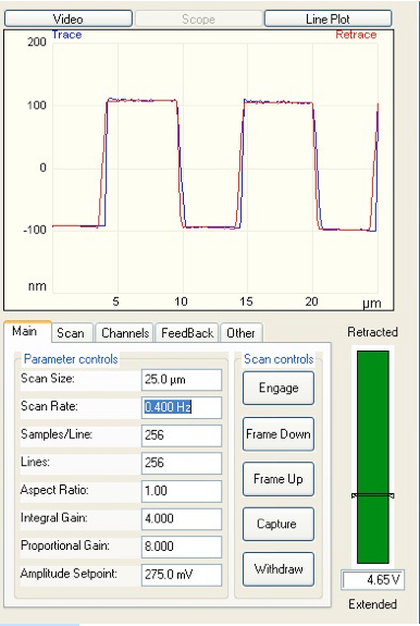
Figure 22. This is the Main menu list of parameters frequently used for optimizing the image. The listed values in the boxes are good starting points for general imaging.
2. Scan
a. The Scan tab table contains a more detailed parameter list pertaining to the scanning control. This set of parameters contains some duplicates from the Main menu and other parameters that are used occasionally. The following explanations describe the more important minor parameters.
- X,Y Offset – allows offsetting the center of the image: usually used to obtain a magnified image of a small section of a current image. It also is used in placing a pattern in a field during AFM lithography.
- SCAN ANGLE – normally the scan angle is 0 degrees aligned to the long axis of the cantilever to obtain most images. A set angle of 90 degrees is used to obtain data from twisting forces on the cantilever, like lateral friction, etc.
- TIP VELOCITY – calculated from the scan frequency. However, if the tip velocity is input, the scan frequency is calculated from this value.
- SLOW SCAN AXIS – this value can be Enabled or Disabled. Sometimes the Disabled value is chosen to help optimize the scanning parameters while scanning over the same track. This provides tip responses from a consistent surface while parameter change effects are evaluated with respect to image quality.
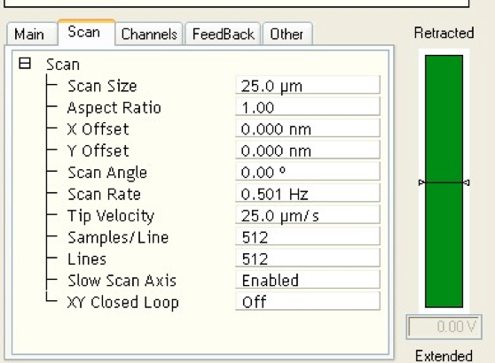
Figure 23. This is the Scan Tab table of nominal parameters. Normally the best images are obtained with the offset set to zero.
3. Channels
a. The Channels tab lists the type of data collected by the AFM. The system can measure 8 parameters at the same time, and this tab allows the user to select and manage the collection conditions for each channel. The following paragraphs describe the parameter settings for normal imaging.
- DATA TYPE – for normal topographical imaging, Height is selected as the primary parameter for channel 1 and Phase is selected for Channel 2. The Phase image looks like the first derivative of the Height data, and the information depicted is related to changes in the “feel’ of the surface, either step height changes (producing bright or dark outlines of features) or surface property changes like hardness, etc.
- DATA SCALE – This is the graph height scale limit usually set in a box under the AFM colored image on the main screen. This tab will copy the number from the main screen. This parameter is used to change the vertical (z) scale on the scope and the color image on the main screen so that a full height image will span the whole vertical scale and show the most detail. It can be changed during a scan if you want to.
- DATA CENTER – Just like the data scale parameter, this one is also set on the main screen under the image and just represents the height offset. i.e. if the image is too dark, you can adjust the Data Center to bring it back to normal.
- The rest of the parameters are just copied from the main screen parameter set under the AFM image.
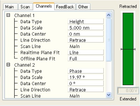
Figure 24. This is the Channels Tab table of nominal starting parameters. There are 8 channels that can collect different data at the same time. Normally the first and second channels are used to capture Height and Phase at the same time.
4. Feedback
a. This tab shows parameters related to the electronic feedback loop that monitors the height of the cantilever through the feedback signal setting the extension or contraction of the Z-Piezo element driving the AFM tip.
- SPM FEEDBACK – for most imaging modes, this feedback signal should be set to “Amplitude.” The rest of the parameters are copies from other tables.
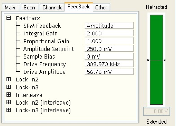
Figure 25. This is the Feedback Tab parameter list. For nominal tapping mode imaging of height, this setting should be Amplitude. NOTE: You can expand or contract the parameter detail list by clicking on the boxed + or -.
5. Other
a. The “Other” tab is a collection of parameters and settings that cover other important settings that didn’t fit in the previous boxes. There are only three parameters that need attention in normal imaging modes: “Microscope mode,” “Z-Range,” and “Units.”
- MICROSCOPE MODE – Sets the mode of operation you want to use; i.e. Tapping Mode, Contact Mode or other.
- Z RANGE – Sets the limits of height. That is, it compresses all the digital measuring points into a designated length maximum. So if your maximum feature height is small, you would reduce this setting to a smaller number encompassing this smaller maximum. That would give you a higher density of height measurement units and thus a higher resolution height image.
- UNITS – Sets the units of height to plot. The default unit is Volts, but normally you would rather have units of distance in Metric units. But before you can have them, you or somebody must have calibrated the metric units to volts. Normally this is done on a regular basis by UTD Cleanroom staff.
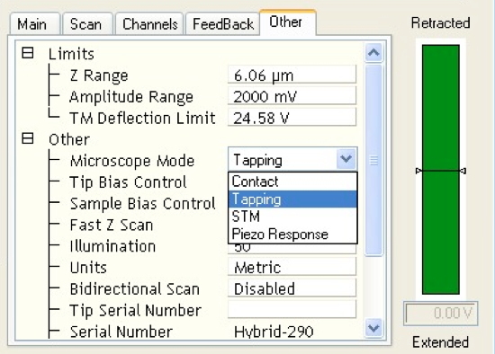
Figure 26. This is the Other Tab listing showing the three most useful parameters in normal height imaging: “Z Range,” “Microscope Mode,” and “Units.”
9. Engage Probe
After you have set all the pertinent parameters described above, and located the place on your sample that you want to image, it is time to “Engage” the tip onto the surface and start scanning. This is executed by pressing the “Engage” button in the list of buttons next to the green graph. The AFM will zip the tip down towards the surface using the “Z-Motor” until it gets close and then it will go very slow, step by step to “feel” for the contact. You can actually hear the Z-motor clicking at each step as it goes into the search region. When it lands it will begin scanning automatically.
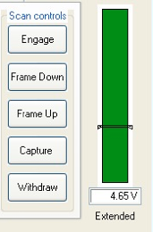
When the tip lands, look at the green bar graph to the right of the Capture button. If the voltage goes to a high number and the graph turns yellow or red, it means that the Z piezo element has extended or contracted to its limit, and you will need to withdraw the tip. ACTION: Click “Withdraw” and then repeat the tip focus and surface focus. Then re-engage. Usually what has happened is that the z-motor has stopped in the wrong place and the z-piezo element could not extend or retract far enough for the tip to actually reach the surface satisfactorily.
Alternatively, you can click on the “Acquire” menu in the toolbar and choose the “Z-Motor” option which will bring up a sub-menu with the option to raise or lower the Z-piezo. Clicking on the up or down boxes will adjust the position of the Z-piezo support so that the Z-piezo element can relax to its center of travel and thus correct the over voltage condition.
10. Adjust Parameters to Optimize Image
Adjusting parameters to optimize the image can be quite involved and tedious. However the normal image optimization can usually be accomplished by adjusting just a few parameters: Scan Rate, Gains (2), and the Amplitude Setpoint.
1. INTEGRAL GAIN: Look at the scope plot of the Trace and Re-Trace (Blue and Red) lines as the tip scans across a topographic feature. The red and blue lines should overlap. If they don’t, for example see Figure 27, then increase the Integral Gain until the amplifier begins to oscillate and produce noise in the trace – then reduce the gain until the noise (oscillations) disappears (Figure 28). What is happening in this case (Figure 27) is that the gain of the amplifier is not sufficient to react to the tip falling into a hole, so the falling edge of both the red and blue traces are quite slanted.
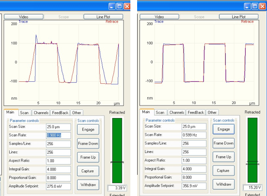
Figure 27. Example of poor overlap between the Trace and Re-Trace profile scans (Left), and better alignment on the right. The Re-Trace (Red) line travels from right to left across the Scope screen and the Blue line goes the other way. Note that the red line falls into the hole too slowly as the AFM tip travels from right to left across the graph, and the Blue re-trace line does the same thing but in the opposite direction. This can be corrected by increasing the gain or slowing the scan rate (right line – image above).
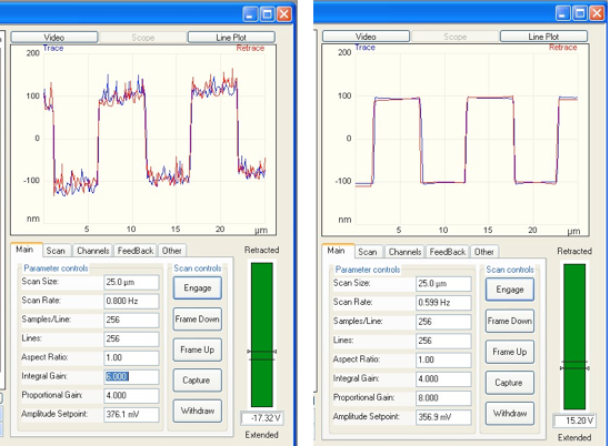
Figure 28. Too much integral gain (Left); just right (Right)
2. PROPORTIONAL GAIN: If the Integral Gain is changed significantly, just make the Proportional Gain twice the amplitude of the Integral Gain.
SCAN RATE: If the gain adjustment does not reunite the overlap of the blue and red trace lines, then try reducing the Scan Rate. This is usually a reliable ploy to overcome the sloped edge problem, but it can slow down the image acquisition time significantly.
3. AMPLITUDE SETPOINT: This is somewhat of a complicated adjustment conceptually. During the cantilever tuning, we set the oscillation amplitude of the cantilever to 500 mV. When the tip landed, the software drove the tip oscillation field into the surface of your sample so that the amplitude dropped to whatever voltage is indicated in the Amplitude Setpoint value window. Sometimes, if the red and blue lines don’t overlap well enough, you can improve things by pressing the left arrow key (with your finger) a few times when the Amplitude Setpoint value box is highlighted. This will reduce the cantilever oscillation amplitude by pushing the oscillating tip closer to the surface and further reducing the oscillation amplitude. This also causes the sharp AFM tip to slam into the material even harder, so be aware of what is going on here and don’t damage the tip or your sample with too much vigor.
11. Capture Image
- Now that you have optimized the image, click on the “Capture” button to record your image. If you look at the very bottom line under the right monitor screen there should be a string of numbers. The “Capture =” number field will indicate the word “next” meaning that the capture will wait until the AFM image completes its current frame and the capture recording will then start when the scan line changes direction and starts the next frame. You can hurry this along by clicking on the “start new frame” icon located in the upper left command line of the left monitor. You can start the frame at either the bottom or top of the frame.
- Once this capture operation has started, if you adjust any parameter, the system will cancel the capture and you will need to restart it manually.
- When the frame scan is complete, the image will appear in your directory of thumbnail images at the right side of the right monitor, and it will be stored in your directory.
12. Save Image
The image is automatically saved to the location you set when you set up the “File path” for saving images.
If you save your image onto the AFM hard drive, remember that the staff has the right to erase images without notice to the owners. This seemingly unreasonable authority is required to keep the AFM running when the disc fills up and locks up the operating system. Therefore, transfer your image to a memory stick as soon as possible so you don’t lose data. Transfer your files using the Windows Explorer program.
13. Shutdown Procedure
- If you have advanced in your experience to the point of performing special operations on the AFM, please reset them to the default values for standard tapping mode operation. Less experienced students may not be able to find the “out-of-adjustment” parameter and will not be able to operate the AFM.
- Withdraw the AFM tip and stop scanning.
- Raise the AFM head about a quarter of an inch (~5 – 10 mm) using the Z-Motor up arrow.
- Move the sample stage away from the head location so that the microscope illumination light and laser spot are left shining on the granite stage.
- Turn off the sample clamping vacuum and remove your sample.
- Screw in the clamping screw for the AFM head and lift it up to remove your AFM scanning tip.
- Replace the AFM head in its dove tail groove.
- Remove the AFM tip from its holder and stash it in your GelPak box.
- Return to the AFM and transfer your images to your memory stick if you have not already stored them there.
- Retrieve your memory stick from the USB port.
- Close the software – click on “File” and “”Exit.
14. Log Out of Logbook
When you are finished with the AFM, sign out of the logbook with the time. Also, the common courtesy is to write “Done” in the logbook to indicate that you have completed your time at the AFM and have gone away. NOTE: If you have encountered a problem during your work, please note its characteristics in the logbook so staff can investigate it.
Appendix A – Summary Listing of AFM Operating Procedures
This listing of AFM instructions is a list of skeletal operating steps designed to give the trained operator a reminder of the order of procedures for Tapping Mode operation.
Step 1. Load the AFM Tip onto the standard holder using the mounting fixture
Step 2. Align and clamp the tip in the holder: Centered and pushed to the back shoulder of the tray
Step 3. Transport the tip in the fixture to the AFM
Step 4. Tighten latch screw on AFM head to loosen head (backward threads)
Step 5. Lift head out of the dove-tail groove and tile upwards to set tip holder onto the four pin mount. Make sure holder is seated flat on pins. Also, do not bend head cables sharply
Step 6. Return AFM head to dove-tail mount and seat it all the way down to the mechanical stop.
Step 7. Loosen the latch screw to tighten the AFM head to its mount.
Step 8. Load your sample onto the air table stage and clamp it down with vacuum (switch on upper panel).
Step 9. Place a white reflective paper (lint free) under the head (on the granite table) so that you can see the microscope illumination circle of light and the red dot from the laser.
Step 10. Start the AFM software to initialize the AFM hardware.
- Double click on the microscope icon on the desktop
- A blank AFM window will open
Step 11. Start your workspace by clicking on “File” in the upper left tool bar and then click on “Open Workspace.”
- Choose your workspace from the “Open” window under
- My Computer
- D40Gb (D:)
- Workspace
- “yourname.wks
- This will install your last saved parameter set
- Workspace
- D40Gb (D:)
- My Computer
Step 12. Click on the yellow microscope icon in the upper left tool bar to initialize the hardware (turn on power, etc.)
- If you see a little window telling you that the stage has not been initialized, click OK to begin initialization. (Make sure that nothing is in the way of the AFM head as it will move to the top of its range.
- Click YES to start initialization
- Click OK to move to top of travel
- Click OK to move optics to end of travel
- Click OK to zoom in
- Click OK to zoom out
Step 13. Open Single Scan window.
Step 14. Click “View’ in the upper left tool bar to open a directory panel – move panel to far right side of the Right screen.
Step 15. Click on the dots-in-a-box icon on the directory panel to select your image directory.
Step 16. Align the AFM head laser to the tip cantilever.
- Use top two “Laser Align” knobs to adjust the location of the red spot under the AFM head on white paper to the right side of the white light circle and then center the shadow of the cantilever in the red laser spot. Note that the green bar graph in “Real Time 1: Meter” window should read ~ 4 – 6 Amplitude units.
Step 17. Center the red dot in the “Real Time 1: Meter” window with the two “Detector Align” knobs on the left side of the AFM head.
Step 18. Load the sample over the appropriate vacuum hole. There are multiple circular groves for vacuum distribution patterns depending of the Sample size and shape.
Step 19. If you have the normal research sized small odd shaped sample, them place it over the center hole in the pattern of 5 holes at the far back of the circular main stage opposite the long tweezers access slot in the stage.
Step 20. Move the stage to position your sample under the AFM head so that the probe tip is positioned over the sample in the appropriate location.
- Click on the “up” arrow in the “RealTime 1: Navigate” window labeled “XY Stage.” This will drive the stage y-motor and move the stage toward the AFM head
- Make sure the head is high enough so the stage or sample will not collide with it.
- If AFM head is too low, raise it by clicking & holding on the up arrow in the
“Z-Motor” sub-window in the navigate window.
Step 21. When the stage is correctly located, lower the AFM head by clicking and holding the “down arrow” in the Z-motor icon. Move the head down until the tip is about 1 mm above your sample.
- Be careful here, you can crash the tip into your sample and damage the AFM. Set the Z-speed to slow (S) when you get close. Stop and get your eyes close to the scan head so you can see the tip position periodically as you perform this operation. When the head arrives at the 1 mm location above the sample, the video screen in the navigate window should be illuminated and you should be able to see your AFM tip in the window.
Step 22. Click on the “Locate Tip” button.
- If the tip is not visible in the window, zoom out some by clicking on the zoom-out arrow.
- Adjust the focus by clicking and holding one of the up down arrows in the “Focus” window (Formerly labeled “Z-Motor”).
- Raise the magnification (Zoom in) to maximum for fine focus – this needs to be an accurate focus.
- If the Tip is not centered near the center of the red cross in the video window, then adjust the Tip position using the two knobs on the optics housing to the left of the AFM head. The point of the tip should be about 5 mm away from the center of the cross for ease of fine focusing.
Step 23. Click on OK when the tip is positioned and in focus. This will change the focus of the
Zoom optics to 1 mm below that of the tip focus.
- The “Focus” window label will change back to “Z-Motor.” Using the slow motor speed setting (S), move the AFM head down until your sample surface is in good focus.
- Note that if you have a polished highly reflective surface, you may not be able to focus on the actual surface. In this case select Tip Reflection from the Focus Surface selection box.
- The Tip Reflection selection will change the focal point of the microscope to 1 mm below the surface in anticipation of focusing on the reflection.
- Note that if you have a polished highly reflective surface, you may not be able to focus on the actual surface. In this case select Tip Reflection from the Focus Surface selection box.
Step 25. Now you need to tune the cantilever oscillation frequency to its resonance point.
- Click on the blue tuning fork icon in the upper left screen tool bar. A big window will overlay the left screen.
- Note: if the tuning fork icon is grayed out, it means that the tapping mode of operation has not been selected.
- To select the tapping mode, open the “Single Scan” window from the Real Time pull-down menu in the upper left command bar.
- Open the “Other” tab in this window and find the “Microscope Mode” selection line.
- Click on the box to the right. It will drop down a list of modes – click on “Tapping.” This will activate the tuning fork icon.
- Note: if the tuning fork icon is grayed out, it means that the tapping mode of operation has not been selected.
- Set tuning parameters
- Set the start and end frequency to span the listed resonance frequency (f0) on the tip box.
- Set the “Target Amplitude’ of the tip oscillation to 500 mV.
- Also check the “Graph” menu and make sure the “Units” parameter is “Metric.”
Step 26. Auto Tune
Click on the “Auto Tune” box to start the tuning process. When it finishes, the “Auto Tune” box will lose its gray tone and you can click on the “Exit’ box. This only takes a few seconds.
Step 27. Software File setup
- This is a good place to set up the file path for saving image data. Pull down the “Real Time” command menu on the command line at the top left of the left screen and click on the Save To… command.
- In the “Save to…” menu box, set the file path to your directory on the D:Imagesyourname directory.
- Then on the View command in the upper left command bar, click on the view directory command. This will place a window on the right side of the right monitor.
- Click on the box containing the 3 dots to call up a window that allows you to select which directory you want to display in this window. Select yours. This is where your images will be saved and you will be able to see a thumbnail of the AFM image there.
- From this thumbnail directory, you can double click on any thumbnail image and call up a new window with the image in the analyze mode so that you can measure x, y and z dimensions as well as statistical roughness.
Step 28. Parameter Setup
At this point you need to set the operation’s main parameters to scan your particular sample. These parameters can vary considerably depending on the nature of your sample. The following parameter settings will work on a hard Silicon-like sample. You will need to adjust them based on your experience with your sample type. The following tables show key parameters that either need adjustment or need to be set for Tapping Mode. There will be many other parameters in the tables, but the listed ones need to be set or checked.
- “Main” tab under “Scan Single” window
| Scan Size | 5 um |
| Scan Rate | 1 Hz |
| Samples/Line | 512 |
| Lines | 512 |
| Aspect Ratio | 1 |
| Integral Gain | 1 |
| Proportional Gain | 2 |
| Amplitude Set Point | 310 |
- “Scan Make sure “Slow Scan Axis” is “Enabled”
- “Channel 1”
| Data Type | Height |
| Line Direction | Retrace |
| Scan Line | Main |
- ”Channel 2”
| Data Type | Phase |
| Line Direction | Retrace |
| Scan Line | Main |
- “Channels 3 – 8”
Data Type Off
- “Feedback” Tab
SPM Feedback Amplitude
- “Other” Tab
| Z-Limit | 6.56 um |
| Microscope Mode | Tapping |
Step 29. Graph Parameters
Options located in boxes under the AFM Image window as quick adjust parameters during real time operation. Most of these have already been set in the “Scan Single” parameter tab settings.
| Data Type | Height | Chanel | 1 | RealtimePlane Fit | Line |
| Scan Line | Main | Data Scale | 400 nm | Offline Plane Fit | Full |
| Line Direction | Retrace | Data Center | 0 | ||
Step 30. Engaging tip (Starting the scan)
- By setting the tip focus and the sample focus in earlier steps, you have set the system conditions required for auto engagement whereby the software automatically lands the tip safely and begins to scan the sample.
- To start this engagement process, click on the “Engage” box. Then wait until the tip starts scanning.
Step 31. Adjustment of initial scanning parameters
- For tapping mode, when the tip begins scanning, watch the “Scope” window where the tip height is plotted against the xy scan. The goal here is to have the Blue Trace line overlap the Red Retrace line.
- If the Blue and Red lines are smooth and separate, it may be that the tip has landed “in air” above the sample. Try highlighting the ”Amplitude Setpoint” value and clicking the left arrow key on the keyboard. This will reduce the amplitude of oscillation of the tip by moving the tip closer to the sample surface. (It may require several arrow clicks…)
- When the scope trace lines show a pattern of consistent wiggles, it means your tip has landed on the surface and you are seeing topography. The more left arrow clicks you execute, the harder the tip hits the surface of your sample.
- If the red and blue trace lines are not overlapping each other, adjust the Integral gain by clicking on the integral gain parameter number and increasing the value.
- If the lines overlap better, keep increasing the gain until the amplifier starts to go into oscillations. Then reduce the gain until the oscillations go away – this is the optimum gain setting.
- Proportional gain does not do much in reality, but the rule of thumb is to set it to twice the numeric value of the Integral gain.
- If the red and blue trace lines still have slanting fall traces after going over steep height changes, then you may need to reduce the scan speed. It is not unusual to drop the speed to something like .5 or .3 Hz.
- If the traces show large “noise,” reduce the integral gain until it calms down.
- If you see regular “herringbone pattern ripples” of color in your AFM image, you most likely have external interference such as electrical or mechanical oscillations from the environment. Try closing the AFM box lid. If this doesn’t eliminate the interference, then call AFM support staff. This may mean that room vibrations have leaked by the vibration damping of the system.
Step 32. Capture Image
- Now that you have optimized the image, click on the “Capture” button to record your image. If you look at the very bottom line under the right monitor screen there should be a string of numbers. The “Capture =” number field will indicate the word “next” meaning that the capture will wait until the AFM image completes its current frame and the capture recording will then start when the scan line changes direction and starts the next frame. You can hurry this along by clicking on the “start new frame” icon located in the upper left command line of the left monitor. You can start the frame at either the bottom or top of the frame.
- Once this capture operation has started, if you adjust any parameter, the system will cancel the capture and you will need to restart it manually.
- When the frame scan is complete, the image will appear in your directory of thumbnail images at the right side of the right monitor, given that you have requested to see it.
Step 33. Analyze Image
- 3D Image Creation
- Click on the thumbnail image in the directory at the right side of the right monitor to open a new window showing that image over in the left monitor space. Highlight the topography image by clicking on it and then click on the 3D icon in the upper left command line to open a new window showing a 3D image. You can manipulate the view of this image with the mouse – see instructions for this in the new window.

- Roughness Measurement
- Highlight the topography window and then click on the roughness icon in the upper left command line. This will bring up a new window with a long list of statistical roughness related parameters. The full window roughness is indicated in the top set of parameters. If you are interested in a small segment of the full image, click and drag open a dotted line rectangle. Then click on the “Execute” button. All the rest of the parameters will then fill in with numbers. The chief roughness results are the Rq and the Ra numbers (Rq=Root Mean Square and Ra=Average Roughness).

- XYZ Measurement of Features
- Highlight the topographical image and click on the “Cross Section” Icon.
- This brings up a new window. In this window, you can draw a line across or through a feature and the box in the upper right of the new window will show the cross section of the feature. In the little window that shows the cross section graph, you can drag cursors out of the edge of the graph wall and position them to measure horizontal or vertical dimensions. The y-axis data comes from drawing a second line over the image feature in a top to bottom direction. Repeat the measurement protocol above for this y-direction line.

- Correction of Slope or Bow
- If your captured image appears to have a slope or bow in it, click on the Flatten icon in the top command line.
- This opens a new window with the ability to make the image plane flat. You can operate on either the entire picture or draw a rectangle around an individual region and flatten just that area. To flatten, click on the Execute button in the right pane of the correction window.

- Reduce Noise in Image
- If your image has lots of “noise” you can reduce it by filtering the noise out. Click on the “Filter” icon in the top row command line.
- This tool also allows you to work on the entire image or just a rectangle you draw with the mouse. Start the filter program by clicking on the Execute button in the right pane of the correction window.
Step 34. Shut down AFM
- Return any special operation settings or parameters to the standard configuration of setting. This is imperative so that the next user who may not be as advanced as you have become can operate the tool after you have gone.
- Withdraw the AFM tip and stop scanning.
- Raise the AFM head about a quarter of an inch (6mm) above the sample stage using the Z-motor up arrow.
- Move the sample stage away from the AFM head so that the microscope illumination light and laser spot are left shining on the granite table.
- Turn off the sample clamping vacuum and remove your sample.
- Screw in the clamping screw for the AFM head and lift it up to remove your AFM scanning tip.
- Replace the AFM head in its dove-tail groove. You need not clamp it there because the next user will want to load his tip.
- Remove the AFM tip from its holder and stash it in your GelPak box.
- Return to the AFM and transfer your images to your memory stick if you have not already done so.
- Retrieve you memory stick from the USB port.
- Close the software
- Log out of the Logbook by entering you completion time. Write “Done” in the comments as courtesy to the next user to let him know that you are finished for sure. NOTE: If you have encountered a problem with the AFM or imaging, please write a note describing the problem. Staff will look at the logbook in the morning and try to fix any problem before the next user arrives.`